Inspect, Sort, Subset and Transform data using Pandas

In this article, we will learn how to inspect data and perform fundamental manipulations, including sorting, subsetting, and transforming data such as creating new columns based on the columns we already have. We will also learn how to combine and apply these skills to answer questions.
Introduction to Pandas
Pandas is a Python package used by data scientists for data manipulation and analysis. We'll start by looking at DataFrames, which is the core of pandas.
Pandas is built on NumPy and Matplotlib
Pandas is built on top of two essential Python packages, NumPy and Matplotlib.
Numpy offers multidimensional array objects for ease of data manipulation, which Pandas takes advantage of to store data, and
Matplotlib boasts powerful data visualization capabilities which pandas makes use of to its advantage.
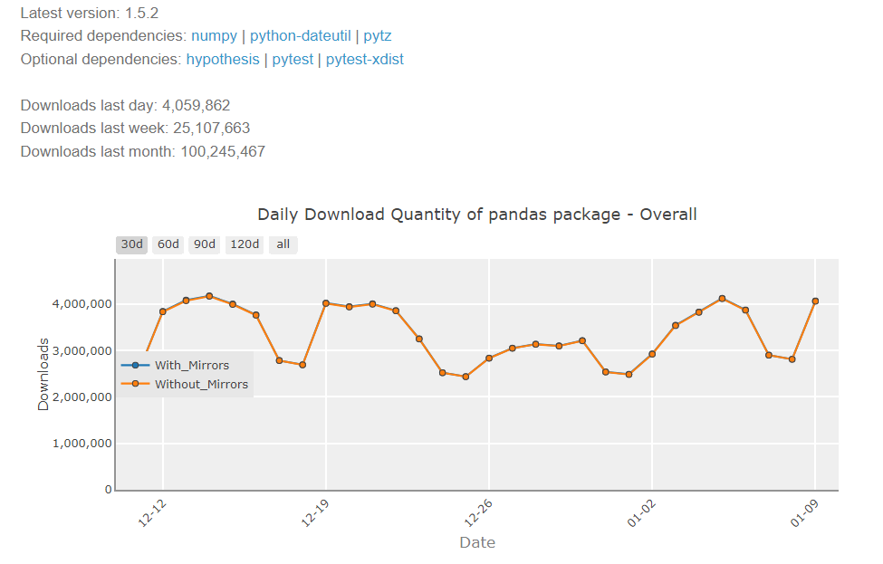
Pandas has millions of users. According to PyPi Stats, Pandas had 100,245,467 downloads during December 2022.
Rectangular or Tabular data structure
There are various structures for storing data for analysis, but the most common and popular is the rectangular data structure, also known as the tabular data structure. Let's import pandas and load the people.csv file which contains data we will use in this article. This people.csv file is available in PyProDev's repository.
import pandas as pd
print('Using pandas version:', pd.__version__)
output:
Using pandas version: 1.3.5
#load data
people = pd.read_csv('people.csv')
print(people)
output:
         Name  Gender Skin Color  Height(cm)  Weight(kg) Date of Birth
0     Michael    Male      Black         175          64    1993-07-29
1      Joseph    Male      Black         180         132    1999-08-27
2     Matthew    Male      Black         162          91    1999-11-05
3      Olivia  Female      Brown         152          47    2003-05-14
4     Madison  Female      Black         160         113    1991-06-13
5       Emily  Female      White         175         104    1992-02-29
6      Amelia  Female      White         173          96    1992-12-31
7       Sarah  Female      Black         172          45    1996-10-19
8      Sophia  Female      Black         155          69    2000-08-07
9        Emma  Female      White         157          60    1991-03-22
10  Alexander    Male      Black         147          45    2001-12-29
11     Daniel    Male      Brown         160          64    2001-07-10
12   Samantha  Female      Brown         160          41    1991-10-04
13      James    Male      White         187         118    1995-12-12
14      David    Male      Brown         193         119    1996-11-24
15     Ashley  Female      White         167          50    2000-04-25
16   Isabella  Female      Brown         166          74    1999-09-13
17    William    Male      White         152          64    1993-09-16
18      Ethan    Male      White         160          41    1998-06-19
19   Benjamin    Male      Brown         170          50    1997-06-06
In this example with people dataset,
each observation or each person is a row, and
each variable, or each person's property, is a column.
pandas is designed to work with rectangular data like this.
pandas DataFrames
Pandas represents rectangular data as a DataFrame object. Similarly, every programming language utilized for data analysis has a similar structure. The values within each column have the same data type, whether numeric or text or object, however, different columns can be different data types.
print(type(people))
output:
<class 'pandas.core.frame.DataFrame'>
Inspecting a DataFrame
When we get a new dataset to work with, the first thing we need to do is explore it and get an idea of what it contains. pandas has several useful methods and attributes for this.
.head()returns the first few rows of the DataFrame..info()shows the information of each of the columns..shapereturns the number of rows and columns of the DataFrame..describe()calculates a few summary statistics for each numeric column.
Exploring a DataFrame using head() method
head() method returns the first few rows of the DataFrame. This becomes very useful if we have many rows.
print(people.head())
output:
      Name  Gender Skin Color  Height(cm)  Weight(kg) Date of Birth
0  Michael    Male      Black         175          64    1993-07-29
1   Joseph    Male      Black         180         132    1999-08-27
2  Matthew    Male      Black         162          91    1999-11-05
3   Olivia  Female      Brown         152          47    2003-05-14
4  Madison  Female      Black         160         113    1991-06-13
Exploring a DataFrame using info() method
The info() method displays the names of columns, the data types they contain, and whether they have any missing values.
print(people.info())
output:
<class 'pandas.core.frame.DataFrame'>
RangeIndex: 20 entries, 0 to 19
Data columns (total 6 columns):
 #   Column         Non-Null Count  Dtype
---  ------         --------------  -----
 0   Name           20 non-null     object
 1   Gender         20 non-null     object
 2   Skin Color     20 non-null     object
 3   Height(cm)     20 non-null     int64
 4   Weight(kg)     20 non-null     int64
 5   Date of Birth  20 non-null     object
dtypes: int64(2), object(4)
memory usage: 1.1+ KB
Exploring a DataFrame using shape attribute
A DataFrame's shape attribute contains a tuple that holds the number of rows followed by the number of columns. Since this is an attribute instead of a method, we write it without parentheses.
print(people.shape)
output:
(20, 6)
Exploring a DataFrame using describe() method
The describe() method computes some summary statistics for numerical columns, like mean and median. "count" is the number of non-missing values in each column. describe() is good for a quick overview of numeric columns.
print(people.describe())
output:
       Height(cm)  Weight(kg)
count   20.000000   20.000000
mean   166.150000   74.350000
std     12.018735   29.716689
min    147.000000   41.000000
25%    159.250000   49.250000
50%    164.000000   64.000000
75%    173.500000   98.000000
max    193.000000  132.000000
Insightful inspecting! We can see that the average height of persons in our dataset is around 166cm. Let's explore the DataFrame further.
Components of a DataFrame
To better understand DataFrame objects, it's useful to know that they consist of three components, stored as attributes.
index: A list of either row numbers or row names.columns: A list of column names.values: A two-dimensional NumPy array of values.
index attribute
The index attribute contains row numbers or row names. Note that row labels are stored in dot-index, not in dot-rows and they are Index objects. This allows for flexibility in labels. For example, our people DataFrame uses row numbers, but row names are also possible. We can usually think of indexes as a list of strings or numbers.
print(people.index)
output:
RangeIndex(start=0, stop=20, step=1)
columns attribute
The columns attribute contains column names.
print(people.columns)
output:
Index(['Name', 'Gender', 'Skin Color', 'Height(cm)', 'Weight(kg)', 'Date of Birth'], dtype='object')
values attribute
The values attribute contains the data values in a 2-dimensional NumPy array.
print(type(people.values))
print(people.values)
output:
<class 'numpy.ndarray'>
[['Michael' 'Male' 'Black' 175 64 '1993-07-29']
 ['Joseph' 'Male' 'Black' 180 132 '1999-08-27']
 ['Matthew' 'Male' 'Black' 162 91 '1999-11-05']
 ['Olivia' 'Female' 'Brown' 152 47 '2003-05-14']
 ['Madison' 'Female' 'Black' 160 113 '1991-06-13']
 ['Emily' 'Female' 'White' 175 104 '1992-02-29']
 ['Amelia' 'Female' 'White' 173 96 '1992-12-31']
 ['Sarah' 'Female' 'Black' 172 45 '1996-10-19']
 ['Sophia' 'Female' 'Black' 155 69 '2000-08-07']
 ['Emma' 'Female' 'White' 157 60 '1991-03-22']
 ['Alexander' 'Male' 'Black' 147 45 '2001-12-29']
 ['Daniel' 'Male' 'Brown' 160 64 '2001-07-10']
 ['Samantha' 'Female' 'Brown' 160 41 '1991-10-04']
 ['James' 'Male' 'White' 187 118 '1995-12-12']
 ['David' 'Male' 'Brown' 193 119 '1996-11-24']
 ['Ashley' 'Female' 'White' 167 50 '2000-04-25']
 ['Isabella' 'Female' 'Brown' 166 74 '1999-09-13']
 ['William' 'Male' 'White' 152 64 '1993-09-16']
 ['Ethan' 'Male' 'White' 160 41 '1998-06-19']
 ['Benjamin' 'Male' 'Brown' 170 50 '1997-06-06']]
Pandas' Swiss Army Knife Philosophy
Python has a philosophy on how to write good code called The Zen of Python. The 13th line of The Zen of Python state that
There should be one-- and preferably only one --obvious way to do it.
This suggestion is that given a programming problem, there should only be one obvious solution. Bear in mind that pandas deliberately doesn't follow this philosophy. Instead, there are often multiple ways to solve a problem, leaving us to choose the best suitable one for us. In this aspect, pandas is like a Swiss Army Knife, giving us a variety of tools, making it incredibly powerful. In this article, we will see a more streamlined standard approach to pandas, only covering the most important ways of doing things.
Sorting and subsetting
Next, we'll learn the two simplest and possibly most important ways, sorting and subsetting, to find interesting parts of our dataset.
Sorting
Finding interesting parts of data in a DataFrame is often easier if we change the order of the rows. The first thing we can do is change the order of the rows by sorting them so that the most interesting data is at the top of the DataFrame. We can sort rows using the sort_values() method, passing in a column name that we want to sort by. For example, when we apply sort_values() on the Weight(kg) column of the people DataFrame, we get the lightest person at the top and the heaviest person at the bottom.
print(people.sort_values('Weight(kg)'))
output:
         Name  Gender Skin Color  Height(cm)  Weight(kg) Date of Birth
12   Samantha  Female      Brown         160          41    1991-10-04
18      Ethan    Male      White         160          41    1998-06-19
10  Alexander    Male      Black         147          45    2001-12-29
7       Sarah  Female      Black         172          45    1996-10-19
3      Olivia  Female      Brown         152          47    2003-05-14
19   Benjamin    Male      Brown         170          50    1997-06-06
15     Ashley  Female      White         167          50    2000-04-25
9        Emma  Female      White         157          60    1991-03-22
11     Daniel    Male      Brown         160          64    2001-07-10
17    William    Male      White         152          64    1993-09-16
0     Michael    Male      Black         175          64    1993-07-29
8      Sophia  Female      Black         155          69    2000-08-07
16   Isabella  Female      Brown         166          74    1999-09-13
2     Matthew    Male      Black         162          91    1999-11-05
6      Amelia  Female      White         173          96    1992-12-31
5       Emily  Female      White         175         104    1992-02-29
4     Madison  Female      Black         160         113    1991-06-13
13      James    Male      White         187         118    1995-12-12
14      David    Male      Brown         193         119    1996-11-24
1      Joseph    Male      Black         180         132    1999-08-27
Sorting in descending order
Setting the ascending argument to False will sort the data the other way around, from the heaviest person to the lightest person.
print(people.sort_values('Weight(kg)', ascending=False))
output:
         Name  Gender Skin Color  Height(cm)  Weight(kg) Date of Birth
1      Joseph    Male      Black         180         132    1999-08-27
14      David    Male      Brown         193         119    1996-11-24
13      James    Male      White         187         118    1995-12-12
4     Madison  Female      Black         160         113    1991-06-13
5       Emily  Female      White         175         104    1992-02-29
6      Amelia  Female      White         173          96    1992-12-31
2     Matthew    Male      Black         162          91    1999-11-05
16   Isabella  Female      Brown         166          74    1999-09-13
8      Sophia  Female      Black         155          69    2000-08-07
0     Michael    Male      Black         175          64    1993-07-29
17    William    Male      White         152          64    1993-09-16
11     Daniel    Male      Brown         160          64    2001-07-10
9        Emma  Female      White         157          60    1991-03-22
15     Ashley  Female      White         167          50    2000-04-25
19   Benjamin    Male      Brown         170          50    1997-06-06
3      Olivia  Female      Brown         152          47    2003-05-14
7       Sarah  Female      Black         172          45    1996-10-19
10  Alexander    Male      Black         147          45    2001-12-29
12   Samantha  Female      Brown         160          41    1991-10-04
18      Ethan    Male      White         160          41    1998-06-19
Sorting by multiple columns
In cases where rows have the same value, we may wish to break the ties by sorting on another column. we can sort based on multiple columns by passing a list of column names in the order of which columns we want to be sorted first. Here, we sort first by weight, then by height.
print(people.sort_values(['Weight(kg)', 'Height(cm)']))
output:
         Name  Gender Skin Color  Height(cm)  Weight(kg) Date of Birth
12   Samantha  Female      Brown         160          41    1991-10-04
18      Ethan    Male      White         160          41    1998-06-19
10  Alexander    Male      Black         147          45    2001-12-29
7       Sarah  Female      Black         172          45    1996-10-19
3      Olivia  Female      Brown         152          47    2003-05-14
15     Ashley  Female      White         167          50    2000-04-25
19   Benjamin    Male      Brown         170          50    1997-06-06
9        Emma  Female      White         157          60    1991-03-22
17    William    Male      White         152          64    1993-09-16
11     Daniel    Male      Brown         160          64    2001-07-10
0     Michael    Male      Black         175          64    1993-07-29
8      Sophia  Female      Black         155          69    2000-08-07
16   Isabella  Female      Brown         166          74    1999-09-13
2     Matthew    Male      Black         162          91    1999-11-05
6      Amelia  Female      White         173          96    1992-12-31
5       Emily  Female      White         175         104    1992-02-29
4     Madison  Female      Black         160         113    1991-06-13
13      James    Male      White         187         118    1995-12-12
14      David    Male      Brown         193         119    1996-11-24
1      Joseph    Male      Black         180         132    1999-08-27
Now, William, Daniel and Michael, are ordered from shortest to tallest, even though they all have the same weight 64 kg. To change the direction values are sorted in, pass a list to the ascending argument to specify which direction sorting should be done for each variable.
print(people.sort_values(['Weight(kg)', 'Height(cm)'], ascending=[True, False]))
output:
         Name  Gender Skin Color  Height(cm)  Weight(kg) Date of Birth
12   Samantha  Female      Brown         160          41    1991-10-04
18      Ethan    Male      White         160          41    1998-06-19
7       Sarah  Female      Black         172          45    1996-10-19
10  Alexander    Male      Black         147          45    2001-12-29
3      Olivia  Female      Brown         152          47    2003-05-14
19   Benjamin    Male      Brown         170          50    1997-06-06
15     Ashley  Female      White         167          50    2000-04-25
9        Emma  Female      White         157          60    1991-03-22
0     Michael    Male      Black         175          64    1993-07-29
11     Daniel    Male      Brown         160          64    2001-07-10
17    William    Male      White         152          64    1993-09-16
8      Sophia  Female      Black         155          69    2000-08-07
16   Isabella  Female      Brown         166          74    1999-09-13
2     Matthew    Male      Black         162          91    1999-11-05
6      Amelia  Female      White         173          96    1992-12-31
5       Emily  Female      White         175         104    1992-02-29
4     Madison  Female      Black         160         113    1991-06-13
13      James    Male      White         187         118    1995-12-12
14      David    Male      Brown         193         119    1996-11-24
1      Joseph    Male      Black         180         132    1999-08-27
Now, Michael, Daniel and William are ordered from tallest to shortest.
Sorting by date
We can use the sort_values() method of pandas to sort data based on date. pandas automatically recognizes and handles date properties for us.
print(people.sort_values('Date of Birth'))
output:
         Name  Gender Skin Color  Height(cm)  Weight(kg) Date of Birth
9        Emma  Female      White         157          60    1991-03-22
4     Madison  Female      Black         160         113    1991-06-13
12   Samantha  Female      Brown         160          41    1991-10-04
5       Emily  Female      White         175         104    1992-02-29
6      Amelia  Female      White         173          96    1992-12-31
0     Michael    Male      Black         175          64    1993-07-29
17    William    Male      White         152          64    1993-09-16
13      James    Male      White         187         118    1995-12-12
7       Sarah  Female      Black         172          45    1996-10-19
14      David    Male      Brown         193         119    1996-11-24
19   Benjamin    Male      Brown         170          50    1997-06-06
18      Ethan    Male      White         160          41    1998-06-19
1      Joseph    Male      Black         180         132    1999-08-27
16   Isabella  Female      Brown         166          74    1999-09-13
2     Matthew    Male      Black         162          91    1999-11-05
15     Ashley  Female      White         167          50    2000-04-25
8      Sophia  Female      Black         155          69    2000-08-07
11     Daniel    Male      Brown         160          64    2001-07-10
10  Alexander    Male      Black         147          45    2001-12-29
3      Olivia  Female      Brown         152          47    2003-05-14
Subsetting
Sometimes we may only want to focus on a specific part of the data instead of the entire data set. This is where subsetting comes in handy.
Subsetting columns
When working with data, we may not need all of the columns in our dataset. We may want to zoom in on just one column. We can do this using the name of the DataFrame, followed by square brackets with a column name inside. Here, we can look at just the Name column.
print(people['Name'])
output:
0       Michael
1        Joseph
2       Matthew
3        Olivia
4       Madison
5         Emily
6        Amelia
7         Sarah
8        Sophia
9          Emma
10    Alexander
11       Daniel
12     Samantha
13        James
14        David
15       Ashley
16     Isabella
17      William
18        Ethan
19     Benjamin
Name: Name, dtype: object
Subsetting multiple columns
To select multiple columns, we need to use two pairs of square brackets. The inner and outer square brackets have different functions. The outer square brackets are used for subsetting the DataFrame, and the inner square brackets are used for creating a list of column names to subset.
print(people[['Name', 'Height(cm)']])
output:
         Name  Height(cm)
0     Michael         175
1      Joseph         180
2     Matthew         162
3      Olivia         152
4     Madison         160
5       Emily         175
6      Amelia         173
7       Sarah         172
8      Sophia         155
9        Emma         157
10  Alexander         147
11     Daniel         160
12   Samantha         160
13      James         187
14      David         193
15     Ashley         167
16   Isabella         166
17    William         152
18      Ethan         160
19   Benjamin         170
This means we can provide a separate list of column names as a variable and then use that list to perform the same subsetting. Usually, it's easier to do in one line.
columns_we_want = ['Name', 'Height(cm)']
print(people[columns_we_want])
output:
         Name  Height(cm)
0     Michael         175
1      Joseph         180
2     Matthew         162
3      Olivia         152
4     Madison         160
5       Emily         175
6      Amelia         173
7       Sarah         172
8      Sophia         155
9        Emma         157
10  Alexander         147
11     Daniel         160
12   Samantha         160
13      James         187
14      David         193
15     Ashley         167
16   Isabella         166
17    William         152
18      Ethan         160
19   Benjamin         170
Subsetting rows on logical conditions
A significant part of data science is recognizing which parts of our dataset are relevant. One of the simplest techniques for this is to find a subset of rows that fulfill certain conditions. This is often referred to as filtering or selecting rows. There are various methods for subsetting a DataFrame, but the most popular is using relational operators to return True or False for each row and then passing that inside square brackets. For example, let's find all the people whose height is greater than 165 centimeters.
rows_we_want = people['Height(cm)'] > 165
print(rows_we_want)
output:
0      True
1      True
2     False
3     False
4     False
5      True
6      True
7      True
8     False
9     False
10    False
11    False
12    False
13     True
14     True
15     True
16     True
17    False
18    False
19     True
Name: Height(cm), dtype: bool
Now we have a True or False value for every row. Then we can use the logical condition inside of square brackets to subset the rows we're interested in to get all of the persons taller than 165 centimeters.
print(people[rows_we_want])
output:
        Name  Gender Skin Color  Height(cm)  Weight(kg) Date of Birth
0    Michael    Male      Black         175          64    1993-07-29
1     Joseph    Male      Black         180         132    1999-08-27
5      Emily  Female      White         175         104    1992-02-29
6     Amelia  Female      White         173          96    1992-12-31
7      Sarah  Female      Black         172          45    1996-10-19
13     James    Male      White         187         118    1995-12-12
14     David    Male      Brown         193         119    1996-11-24
15    Ashley  Female      White         167          50    2000-04-25
16  Isabella  Female      Brown         166          74    1999-09-13
19  Benjamin    Male      Brown         170          50    1997-06-06
Subsetting based on string
We can also subset rows based on text data, string. Here, we use the double equal sign in the logical condition to filter the people who are males.
rows_to_keep = people['Gender'] == 'Male'
print(people[rows_to_keep])
         Name Gender Skin Color  Height(cm)  Weight(kg) Date of Birth
0     Michael   Male      Black         175          64    1993-07-29
1      Joseph   Male      Black         180         132    1999-08-27
2     Matthew   Male      Black         162          91    1999-11-05
10  Alexander   Male      Black         147          45    2001-12-29
11     Daniel   Male      Brown         160          64    2001-07-10
13      James   Male      White         187         118    1995-12-12
14      David   Male      Brown         193         119    1996-11-24
17    William   Male      White         152          64    1993-09-16
18      Ethan   Male      White         160          41    1998-06-19
19   Benjamin   Male      Brown         170          50    1997-06-06
Subsetting based on dates
We can also subset based on dates. Here, we filter all the persons born before year 2000. Notice that the dates are written as year then month, then day. This is the international standard date format.
rows_we_want = people['Date of Birth'] < '2000-01-01'
print(people[rows_we_want])
output:
        Name  Gender Skin Color  Height(cm)  Weight(kg) Date of Birth
0    Michael    Male      Black         175          64    1993-07-29
1     Joseph    Male      Black         180         132    1999-08-27
2    Matthew    Male      Black         162          91    1999-11-05
4    Madison  Female      Black         160         113    1991-06-13
5      Emily  Female      White         175         104    1992-02-29
6     Amelia  Female      White         173          96    1992-12-31
7      Sarah  Female      Black         172          45    1996-10-19
9       Emma  Female      White         157          60    1991-03-22
12  Samantha  Female      Brown         160          41    1991-10-04
13     James    Male      White         187         118    1995-12-12
14     David    Male      Brown         193         119    1996-11-24
16  Isabella  Female      Brown         166          74    1999-09-13
17   William    Male      White         152          64    1993-09-16
18     Ethan    Male      White         160          41    1998-06-19
19  Benjamin    Male      Brown         170          50    1997-06-06
Subsetting based on multiple logical conditions
In order to subset the rows that meet multiple conditions, we can use logical operators, such as the "and" operator, &, to combine the conditions. This ensures that only rows that satisfy both of these conditions will be subsetted.
is_male = people['Gender'] == 'Male'
is_brown = people['Skin Color'] == 'Brown'
print(people[is_male & is_brown])
output:
        Name Gender Skin Color  Height(cm)  Weight(kg) Date of Birth
11    Daniel   Male      Brown         160          64    2001-07-10
14     David   Male      Brown         193         119    1996-11-24
19  Benjamin   Male      Brown         170          50    1997-06-06
We can also do this in one line of code, but we'll also need to add parentheses around each condition.
print(people[(people['Gender'] == 'Male') & (people['Skin Color'] == 'Brown')])
output:
        Name Gender Skin Color  Height(cm)  Weight(kg) Date of Birth
11    Daniel   Male      Brown         160          64    2001-07-10
14     David   Male      Brown         193         119    1996-11-24
19  Benjamin   Male      Brown         170          50    1997-06-06
Using square brackets plus logical conditions is often the most powerful way of identifying interesting rows of data.
Subsetting by categorical columns
When trying to subset data based on multiple values of a categorical column, we use the "or" operator, |, to select rows from multiple categories. However, this can become tedious when dealing with many categorical values. A more efficient method is to use the .isin() method, which accepts a list of values to filter for. Here, we check if the color of a person is black or brown, and use this condition to subset the data.
is_black_or_brown = people['Skin Color'].isin(['Black', 'Brown'])
print(people[is_black_or_brown])
output:
         Name  Gender Skin Color  Height(cm)  Weight(kg) Date of Birth
0     Michael    Male      Black         175          64    1993-07-29
1      Joseph    Male      Black         180         132    1999-08-27
2     Matthew    Male      Black         162          91    1999-11-05
3      Olivia  Female      Brown         152          47    2003-05-14
4     Madison  Female      Black         160         113    1991-06-13
7       Sarah  Female      Black         172          45    1996-10-19
8      Sophia  Female      Black         155          69    2000-08-07
10  Alexander    Male      Black         147          45    2001-12-29
11     Daniel    Male      Brown         160          64    2001-07-10
12   Samantha  Female      Brown         160          41    1991-10-04
14      David    Male      Brown         193         119    1996-11-24
16   Isabella  Female      Brown         166          74    1999-09-13
19   Benjamin    Male      Brown         170          50    1997-06-06
Using .isin() makes subsetting by categorical variables a breeze.
Transforming data
We learned how to subset and sort a DataFrame to extract relevant information. However, it is often the case that the contents of a DataFrame do not meet our needs when first received. Thankfully, we are not stuck with the data provided to us. We can create new columns from scratch, but it is also common to create new columns derived from existing columns. For example, by adding columns together or by changing their units. Transforming data and adding new columns can go by many names, including
mutating a DataFrame or
transforming a DataFrame or
feature engineering.
To add a new column to our DataFrame that has each person's height in meters, instead of centimeters, we use square brackets with the name of the new column we want to create on the left-hand side of the equals sign. On the right-hand side, we have the calculation. It's worth noting that both the existing column and the new column we just created are now in the DataFrame.
people['Height(m)'] = people['Height(cm)'] / 100
display(people)
| Name | Gender | Skin Color | Height(cm) | Weight(kg) | Date of Birth | Height(m) | |
| 0 | Michael | Male | Black | 175 | 64 | 1993-07-29 | 1.75 |
| 1 | Joseph | Male | Black | 180 | 132 | 1999-08-27 | 1.80 |
| 2 | Matthew | Male | Black | 162 | 91 | 1999-11-05 | 1.62 |
| 3 | Olivia | Female | Brown | 152 | 47 | 2003-05-14 | 1.52 |
| 4 | Madison | Female | Black | 160 | 113 | 1991-06-13 | 1.60 |
| 5 | Emily | Female | White | 175 | 104 | 1992-02-29 | 1.75 |
| 6 | Amelia | Female | White | 173 | 96 | 1992-12-31 | 1.73 |
| 7 | Sarah | Female | Black | 172 | 45 | 1996-10-19 | 1.72 |
| 8 | Sophia | Female | Black | 155 | 69 | 2000-08-07 | 1.55 |
| 9 | Emma | Female | White | 157 | 60 | 1991-03-22 | 1.57 |
| 10 | Alexander | Male | Black | 147 | 45 | 2001-12-29 | 1.47 |
| 11 | Daniel | Male | Brown | 160 | 64 | 2001-07-10 | 1.60 |
| 12 | Samantha | Female | Brown | 160 | 41 | 1991-10-04 | 1.60 |
| 13 | James | Male | White | 187 | 118 | 1995-12-12 | 1.87 |
| 14 | David | Male | Brown | 193 | 119 | 1996-11-24 | 1.93 |
| 15 | Ashley | Female | White | 167 | 50 | 2000-04-25 | 1.67 |
| 16 | Isabella | Female | Brown | 166 | 74 | 1999-09-13 | 1.66 |
| 17 | William | Male | White | 152 | 64 | 1993-09-16 | 1.52 |
| 18 | Ethan | Male | White | 160 | 41 | 1998-06-19 | 1.60 |
| 19 | Benjamin | Male | Brown | 170 | 50 | 1997-06-06 | 1.70 |
Creating new BMI(Boby Mass Index) columns
Let's calculate the body mass index of the people in our DataFrame, we can use the weight and height columns to create a new column that shows the BMI for each person. This is done by dividing weight(kg) by height(m) squared.
$$\text{BMI} = \frac{\text{weight in kg}}{(\text{height in m})^2}$$
Again, the new column is on the left-hand side of the equals, but this time, our calculation involves two columns.
people['BMI'] = people['Weight(kg)'] / people['Height(m)'] ** 2
display(people)
| Name | Gender | Skin Color | Height(cm) | Weight(kg) | Date of Birth | Height(m) | BMI | |
| 0 | Michael | Male | Black | 175 | 64 | 1993-07-29 | 1.75 | 20.897959 |
| 1 | Joseph | Male | Black | 180 | 132 | 1999-08-27 | 1.80 | 40.740741 |
| 2 | Matthew | Male | Black | 162 | 91 | 1999-11-05 | 1.62 | 34.674592 |
| 3 | Olivia | Female | Brown | 152 | 47 | 2003-05-14 | 1.52 | 20.342798 |
| 4 | Madison | Female | Black | 160 | 113 | 1991-06-13 | 1.60 | 44.140625 |
| 5 | Emily | Female | White | 175 | 104 | 1992-02-29 | 1.75 | 33.959184 |
| 6 | Amelia | Female | White | 173 | 96 | 1992-12-31 | 1.73 | 32.075913 |
| 7 | Sarah | Female | Black | 172 | 45 | 1996-10-19 | 1.72 | 15.210925 |
| 8 | Sophia | Female | Black | 155 | 69 | 2000-08-07 | 1.55 | 28.720083 |
| 9 | Emma | Female | White | 157 | 60 | 1991-03-22 | 1.57 | 24.341758 |
| 10 | Alexander | Male | Black | 147 | 45 | 2001-12-29 | 1.47 | 20.824656 |
| 11 | Daniel | Male | Brown | 160 | 64 | 2001-07-10 | 1.60 | 25.000000 |
| 12 | Samantha | Female | Brown | 160 | 41 | 1991-10-04 | 1.60 | 16.015625 |
| 13 | James | Male | White | 187 | 118 | 1995-12-12 | 1.87 | 33.744173 |
| 14 | David | Male | Brown | 193 | 119 | 1996-11-24 | 1.93 | 31.947166 |
| 15 | Ashley | Female | White | 167 | 50 | 2000-04-25 | 1.67 | 17.928215 |
| 16 | Isabella | Female | Brown | 166 | 74 | 1999-09-13 | 1.66 | 26.854406 |
| 17 | William | Male | White | 152 | 64 | 1993-09-16 | 1.52 | 27.700831 |
| 18 | Ethan | Male | White | 160 | 41 | 1998-06-19 | 1.60 | 16.015625 |
| 19 | Benjamin | Male | Brown | 170 | 50 | 1997-06-06 | 1.70 | 17.301038 |
If our dataset doesn't have the exact columns we need, we can often make our own from what we have.
Extract insights through data manipulation
We've seen the most common types of data manipulation:
sorting,
subsetting, and
transforming data.
By utilizing all the techniques we've learned, we can combine them to answer a wide range of questions in a real-life data analysis scenario. Let's find out the names of skinny, tall people. First, to define skinny people, we take the subset of the people who have a BMI of under 19.
bmi_less_than_19 = people[people['BMI'] < 19]
Next, we sort the result in descending order of height to get the tallest skinny persons at the top.
bmi_less_than_19_sortedby_height = bmi_less_than_19.sort_values('Height(cm)', ascending=False)
Finally, we keep only the columns we're interested in. Here, we can see that Sarah is the tallest person with a BMI of under 19.
print(bmi_less_than_19_sortedby_height[['Name','Height(cm)','BMI']])
output:
        Name  Height(cm)        BMI
7      Sarah         172  15.210925
19  Benjamin         170  17.301038
15    Ashley         167  17.928215
12  Samantha         160  16.015625
18     Ethan         160  16.015625
Cool combination! In our dataset, there are 5 persons whose BMIs are under 19 and Sarah is the tallest with 172cm height among these 5 persons.
Conclusion
In this article, we learned how to inspect Data and perform fundamental manipulations, including sorting, subsetting, and transforming data such as creating new columns based on the columns we already have. We also combined and applied these skills to answer who is the tallest skinny person in our people dataset.
#python #pandas #data-science


